Tile-Low-Rank Matrices in NextLA.jl
20 Aug 2026Table of Contents
- Introduction
- My contribution
- Two TLR variants
- Packing variable-rank tiles
- Compression with ARA
- GEMM on compressed operands
- Results
- Using the implementation
- References
Introduction
A dense \(32{,}768 \times 32{,}768\) Float64 matrix costs 8.6 GB to
store, and operations such as factorization still scale cubically in the
matrix dimension. But many matrices that appear in scientific computing do
not contain that much independent information. Boundary element
discretizations, Gaussian process covariance matrices, and kernel matrices
from radial basis functions often have smooth interactions between
well-separated groups of points. Smooth interactions are numerically low
rank, so after blocking the matrix, most off-diagonal tiles have singular
values that decay after only a small number of terms.
The storage arithmetic is already enough to motivate the format. Tile the \(32{,}768 \times 32{,}768\) matrix into \(1024 \times 1024\) blocks. The 32 diagonal tiles stay dense, while the remaining 992 off-diagonal tiles are stored as rank-16 factor pairs. The dense diagonal costs 268 MB, and the off-diagonal factors cost about 260 MB. The result is 528 MB instead of 8.6 GB, about a 16x reduction.
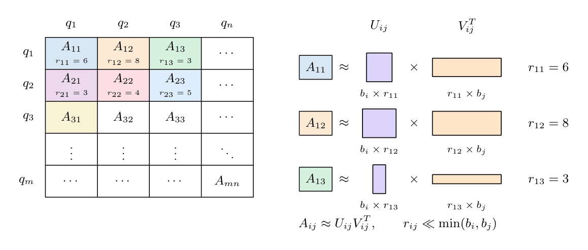
Tile-Low-Rank (TLR) uses that observation directly. Cut the matrix into a flat grid of tiles. Keep the diagonal dense, since it represents the near field and is usually genuinely full rank. Replace each off-diagonal tile with two skinny factors,
\[A_{ij} \approx U_{ij}V_{ij}^{T}, \qquad U_{ij}\in\mathbb{R}^{b_i\times r_{ij}}, \quad V_{ij}\in\mathbb{R}^{b_j\times r_{ij}},\]where \(r_{ij}\) is much smaller than the tile size. Unlike a global low-rank factorization, each tile gets its own rank. Unlike \(\mathcal{H}\)-matrices or HODLR, there is no tree and no recursion: one level, one tile size, and one regular grid. That gives up some compressibility, but it produces a layout that is far easier to schedule on a GPU, which is fundamental for performance in real applications.
During the Google Summer of Code I implemented the TLR module in NextLA.jl, a Julia library aiming to provide next-generation dense linear algebra: mixed precision, low-rank formats, and multiple hardware backends behind one API, on CPU and GPU without hardware-specific code paths. This post describes the TLR module we added.
My contribution
The code is available in NextLA.jl and was introduced in pull request #20.
The main result is an end-to-end public pipeline for working with TLR matrices. Starting from ordinary dense matrices, NextLA can now build compressed representations,
\[A \longrightarrow A_{\mathrm{tlr}}, \qquad B \longrightarrow B_{\mathrm{tlr}},\]where each object stores the matrix by tiles rather than as one dense array.
The API exposes two variants: TLRMatrix, which keeps the diagonal tiles
dense, and CompressedFTLRMatrix, where every tile is stored in compressed
form.
Once the matrices are compressed, they can be used directly in BLAS-like products,
\[C \leftarrow \alpha\,\operatorname{op}(A_{\mathrm{tlr}}) \operatorname{op}(B_{\mathrm{tlr}}) + \beta C,\]with support for TLR × TLR, TLR × dense, and dense × TLR. There is also
an allocation-returning path where the output remains compressed,
so the product does not have to be materialized as a dense matrix. The API also exposes the controls needed for real workloads: transpose combinations, mixed-precision compute modes, workspace limits, and workspace reuse.
Below we illustrate some implementation details and provide a small tutorial to show how to construct the TLR matrices, multiply them, and choose how much precision and memory to spend.
Two TLR variants
We implemented two versions of the format. TLRMatrix follows the usual
scientific-computing layout [1]: diagonal tiles are dense and off-diagonal
tiles are compressed. CompressedFTLRMatrix stores every tile, including the
diagonal, as a factor pair. The second format is useful when there is no clear
dense near field, which is common for blockwise-compressed machine-learning
matrices [4].
Packing variable-rank tiles
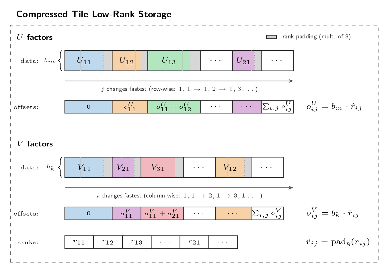
Storing every factor at an operand-wide maximum rank would make the arrays regular, but it would also bring back arithmetic and memory that compression was supposed to remove. NextLA instead stores each tile using its discovered logical rank.
The two factors use complementary traversal orders. The \(U\) factors are
packed by tile row, while the \(V\) factors are packed by tile column. This
makes a row panel of \(U\) and a column panel of \(V\) available as contiguous
views at the same time. Transposition only exchanges the two roles, so the same
storage works for every N/T operand combination without keeping another
copy.
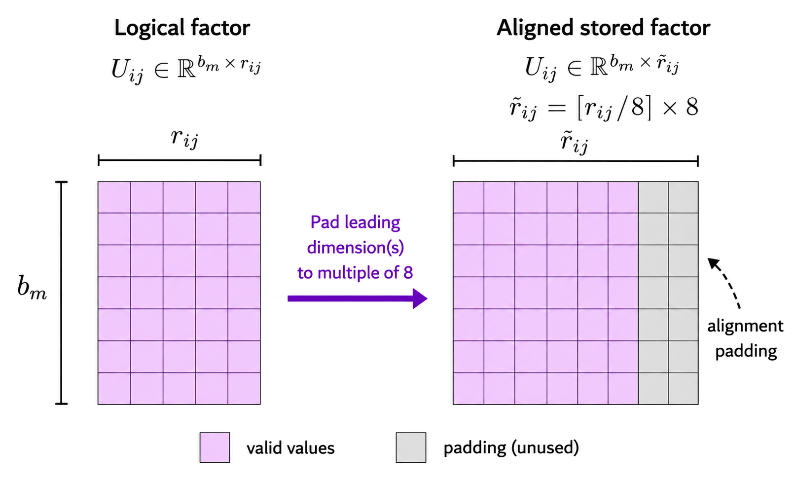
Some low-precision kernels, including grouped GEMM, require aligned factor
addresses and dimensions. The rank_multiple option meets this requirement by
padding each factor’s stored capacity without changing its logical rank, error
estimate, or numerical result. On current CUDA hardware, use
rank_multiple=8 for FP16 and BF16 factors.
Compression with ARA
The tile ranks are outputs of the compression, not inputs. We use Adaptive
Randomized Approximation (ARA) [2] to sample a batch of tiles and grow an
orthogonal basis until each tile meets the requested tolerance or reaches
maxrank.
Tiles in one batch do not necessarily converge together. The implementation therefore keeps separate progress and stopping state for every tile. On each pass it projects a fresh sample against the existing basis, performs two-pass Cholesky QR, and checks the new projected columns. Finished tiles retire while the others continue. A final small SVD chooses the stored rank and records the remaining error.
From the user side, this is just a constructor:
A_tlr = TLRMatrix(A, 256;
                  maxrank=64,
                  tol=1f-5,
                  rel=true,
                  r_required=10)
Here r_required controls how many consecutive negligible samples ARA needs
before declaring a tile converged. Compression workspaces can also be reused
when several matrices have the same shape and tiling.
GEMM on compressed operands
The dense-output interface follows BLAS:
\[C \leftarrow \alpha\,\operatorname{op}(A)\operatorname{op}(B)+\beta C, \qquad \operatorname{op}(X)\in\{X,X^T\}.\]The API covers two compressed operands as well as mixed dense/compressed
products. TLRMatrix also carries dense diagonal tiles and smaller boundary
tiles, so its GEMM combines the compressed off-diagonal product with the two
dense-diagonal cross terms and the diagonal product.
The interesting part is the product of two compressed tiles. Write
\[A_{i\ell}=U_{i\ell}V_{i\ell}^{T}, \qquad B_{\ell j}=W_{\ell j}Z_{\ell j}^{T}.\]Then one output tile is
\[C_{ij}=\sum_{\ell} U_{i\ell}\underbrace{\left(V_{i\ell}^{T}W_{\ell j}\right)}_{S_{i\ell j}} Z_{\ell j}^{T}.\]Computing that expression tile by tile gives many tiny GEMMs and repeatedly loads and stores \(C_{ij}\). Most of the GEMM work went into avoiding that. The packed factors let us fuse adjacent tile rows and columns into larger views, and the product is lowered in three stages:
- form the small coupling matrices \(S_{i\ell j}\);
- multiply \(S\) by one side’s factors;
- fold the sum over \(\ell\) into the reduction dimension of a final GEMM.
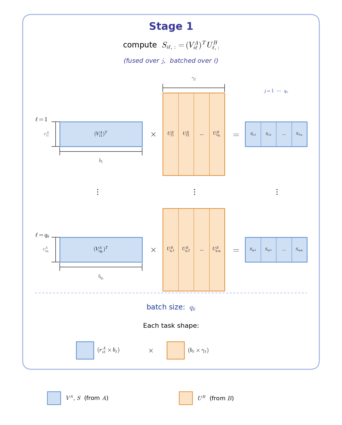
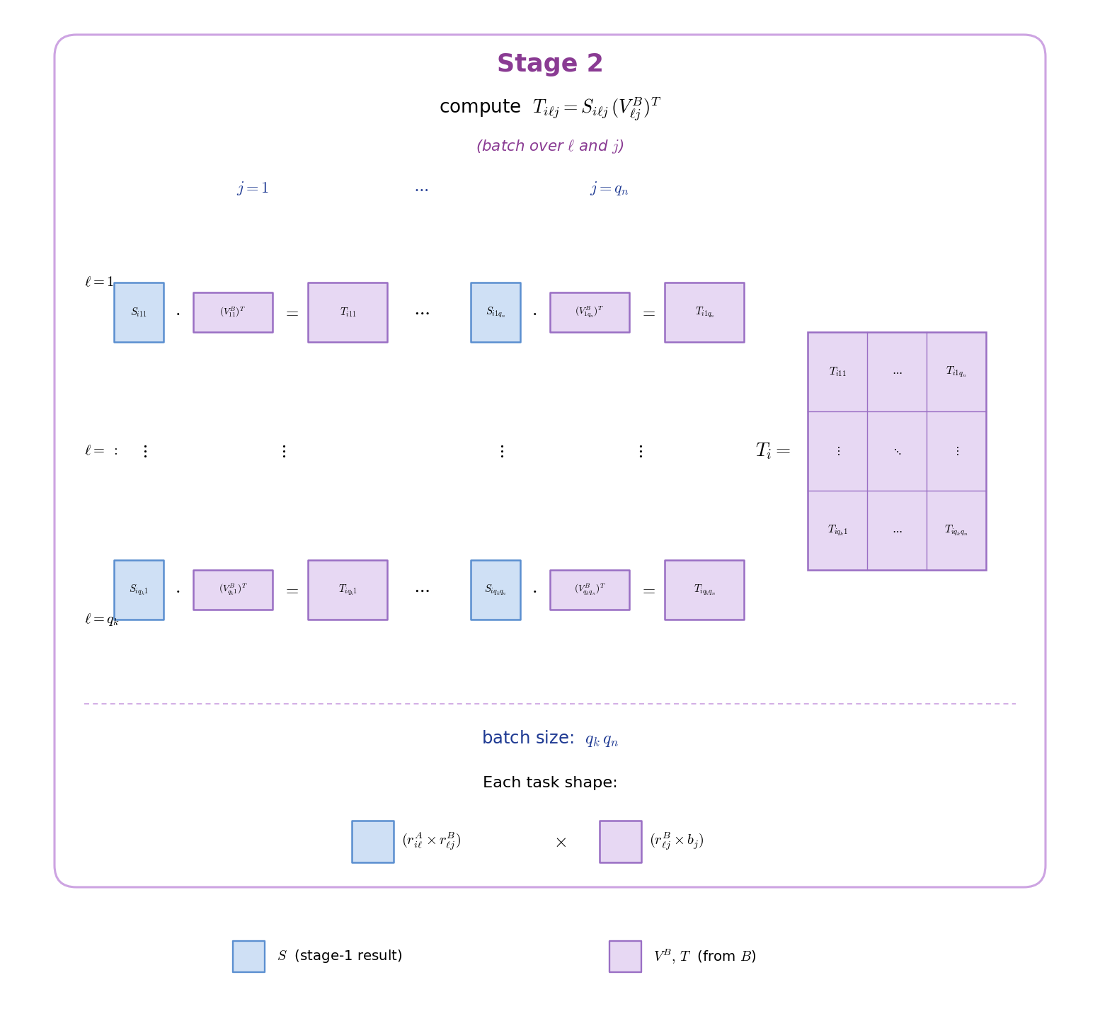
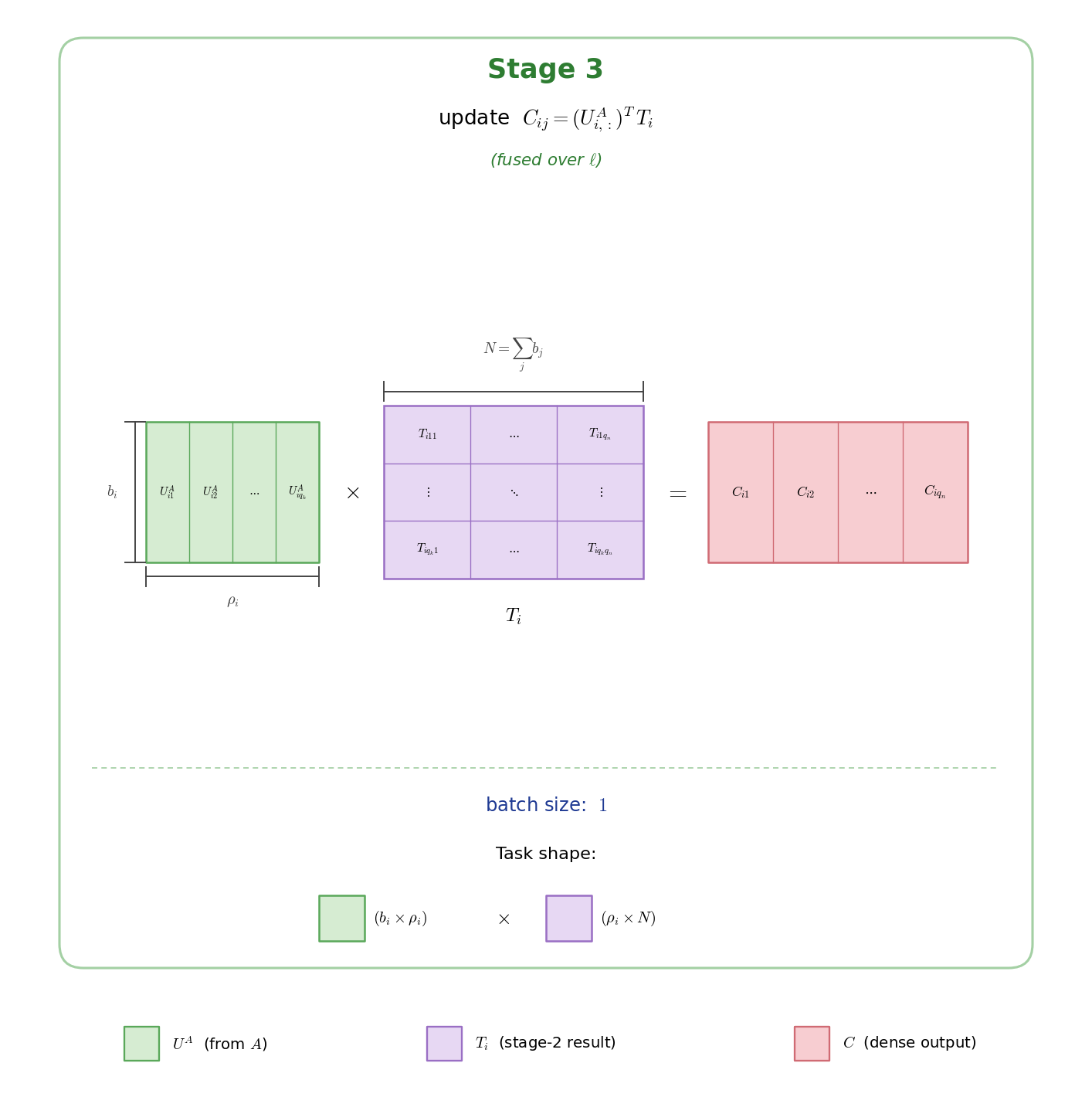
There are two valid contraction orders. FoldRight computes \(U(SZ^T)\); FoldLeft computes \((US)Z^T\). Their temporary sizes and operation counts depend on the ranks in the current rows and columns. The scheduler looks at that rank metadata and chooses the cheaper feasible direction instead of imposing one order on the entire matrix.
Workspace is part of the schedule
The temporary workspace determines how many output tiles can be fused in one run. With more memory, the scheduler builds wider operations. With less, it splits the output into smaller row and column ranges while staying inside the requested byte limit.
NextLA exposes minimum and maximum workspace queries. For fully compressed
operands, gemm_workspace_bytes(A, B; runs=n) chooses the smallest workspace
that meets a target number of runs. The symbolic schedule and prepared
grouped-GEMM descriptors can be cached and reused when the matrix dimensions
and rank distribution stay the same.
This makes the memory/performance tradeoff explicit. A caller can use the fastest schedule when memory is available or deliberately trade some fusion for a smaller peak allocation.
Returning a compressed result
The allocation-returning gemm(A_tlr, B_tlr; ...) keeps the result compressed.
This is a different problem from the dense-output path: the rank of each output
tile is unknown until the product has been sampled. We cannot allocate its
final packed offsets in advance, and forming a dense tile just to compress it
would lose most of the benefit.
For one output tile, define
\[X_{ij}=\alpha\sum_{\ell} A_{i\ell}B_{\ell j} =\alpha\sum_{\ell} U^A_{i\ell}S_{i\ell j}(V^B_{\ell j})^T, \qquad S_{i\ell j}=(V^A_{i\ell})^TU^B_{\ell j}.\]The coupling matrices \(S_{i\ell j}\) depend on the input factors but not on the random samples, so they are computed once for a run and reused. A right sample of the complete tile is then
\[X_{ij}\Omega =\alpha\sum_{\ell}U^A_{i\ell}S_{i\ell j} \left((V^B_{\ell j})^T\Omega\right).\]This is evaluated as three GEMM contractions: project the random block through \(V^B\), apply the small coupling matrices, and reduce all \(\ell\) contributions through the packed \(U^A\) row. The wide \(b_m\times b_n\) tile \(X_{ij}\) never exists in memory. If left sampling is cheaper, the implementation applies the transpose expression instead. Complementary packing provides the contiguous row or column stack needed by either direction and by all four transpose combinations.
ARA repeats this implicit apply with fresh random blocks and grows a basis \(Q\) until the tile converges. It then applies the complementary operator once,
\[Z_{ij}=X_{ij}^TQ_{ij}, \qquad X_{ij}\approx Q_{ij}Z_{ij}^T,\]and performs a small final SVD to select the output rank and split the result into its two stored factors. In contrast to sequential recompression, the whole sum over \(\ell\) is compressed once rather than after every contraction tile.
The output grid is processed with a rolling workspace. A byte budget determines how many ARA slots are available. A fixed-row or fixed-column run fills those slots; when some tiles converge, they are moved to a retired suffix, truncated, and copied to output staging. Pending tiles immediately reuse the freed slots. Workspace therefore scales with the chosen concurrency rather than with the number of output tiles.
During this pass, staging factors have a uniform width of maxrank. Once every
logical rank is known, NextLA allocates the final exact-rank offsets, applies
rank_multiple if alignment is requested, and copies only the active factor
columns. This is why compressed-output GEMM returns a newly allocated matrix
instead of accepting a finalized packed destination through gemm!.
The main controls are:
| Keyword | Role in compressed-output GEMM |
|---|---|
maxrank |
Upper bound for every discovered output rank and the temporary staging width |
tol, rel |
Absolute or relative error target used by final truncation |
eps_rel |
Sampling tolerance for the adaptive range finder; defaults from tol and the numerical stopping floor |
block |
Number of random columns drawn in one ARA pass |
r_required |
Consecutive negligible samples required before a tile retires |
workspace |
Optional byte budget; larger values allow more simultaneous ARA slots |
rank_multiple |
Alignment quantum for the final stored capacities, without changing logical ranks |
The current compressed-output entry point accepts two CompressedFTLRMatrix
operands on a regular tile grid. It supports NN, NT, TN, and TT, plus
the same mixed-precision compute modes as the dense-output implementation.
Results
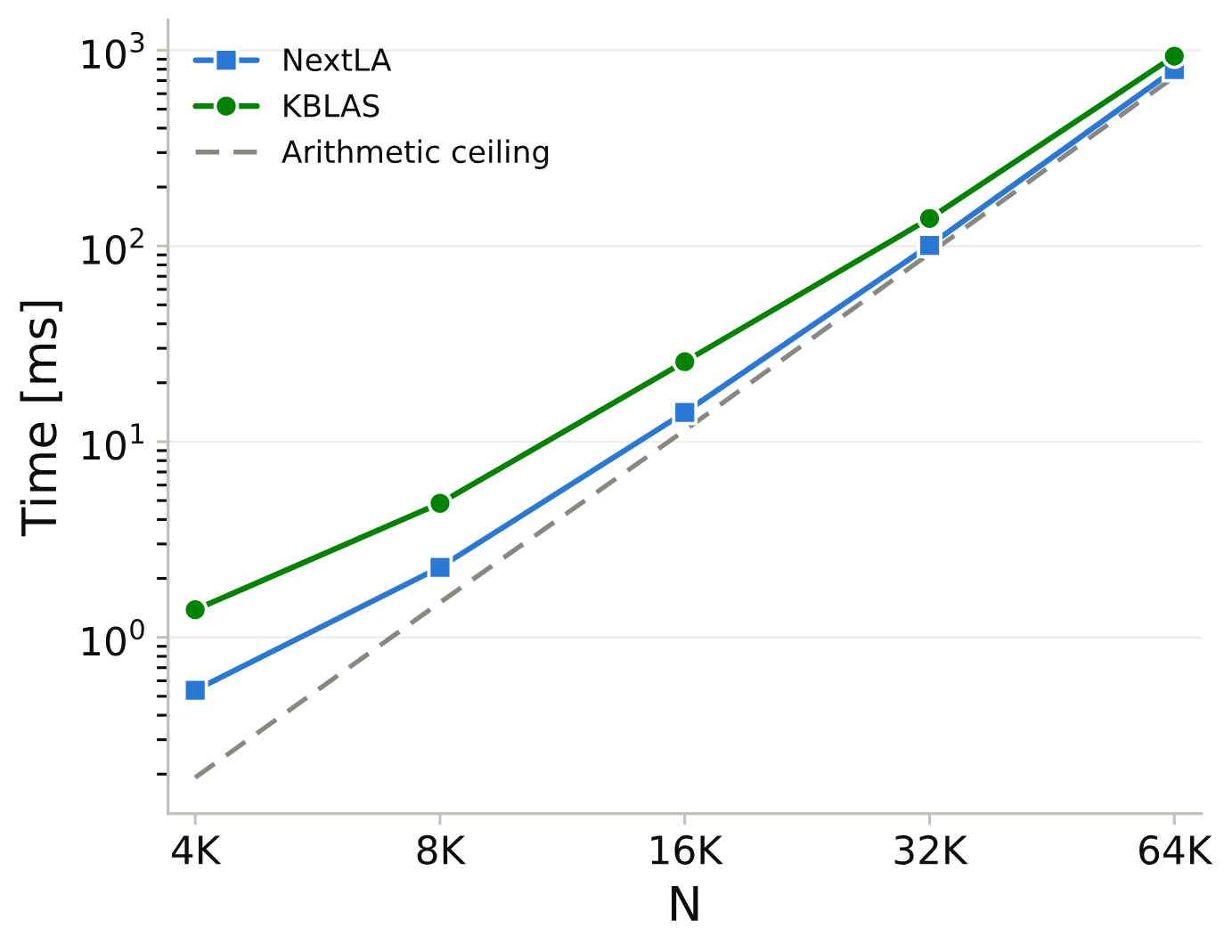
We evaluated the dense-output GEMM on an NVIDIA H100 with both uniform and skewed tile-rank distributions. A direct comparison with KBLAS is necessarily limited: KBLAS supports FP32 and FP64 and uses one common rank for every tile in an operand. NextLA additionally supports BF16, FP16, and TF32 on CUDA, and executes each tile at its own rank.
For constant-rank FP32 problems, NextLA reached 92.1% of the ceiling obtained by scaling dense-GEMM time by the executed-FLOP ratio. On the configurations shared with KBLAS, it was 1.44 times faster in geometric mean and up to 2.58 times faster. The advantage is larger for variable ranks because NextLA does not pad every tile to one operand-wide rank.
The constant-rank experiment above provides the like-for-like KBLAS comparison. The next experiment uses the feature that the padded baseline cannot represent directly: different ranks for different tiles. Each matrix has eight tiles per axis, hence 64 tiles in total, with tile size \(b=N/8\) and ranks varying between \(b/16\) and \(b/8\). The bars report speedup over the corresponding dense GEMM for several matrix sizes and compute modes.
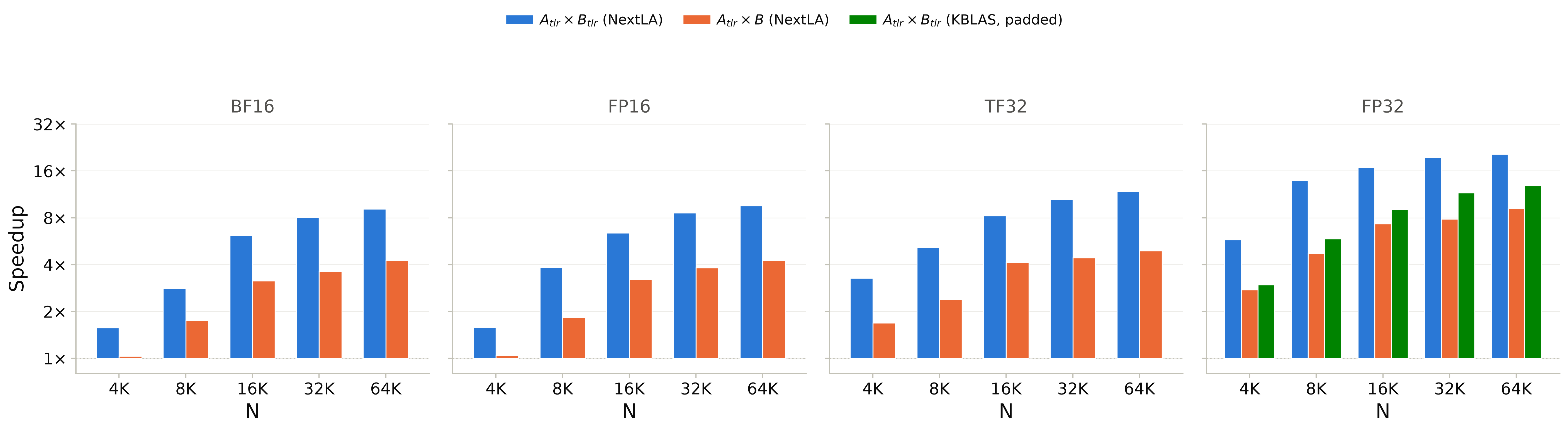
The missing KBLAS bars in the BF16, FP16, and TF32 panels are therefore not omitted measurements; those execution modes are not supported by KBLAS. The NextLA speedup increases with matrix size as the fused compressed operations become large enough to use the GPU efficiently.
The workspace experiments show the other side of the design. One FP16 configuration was 6.34 times faster than dense GEMM while using 17.8% of the dense-input memory. In the largest reported FP16 case, \(N=65{,}536\) completed in 81.8 ms, 9.57 times faster than the dense baseline while using 10.7% of its operand memory.
Using the implementation
Assume A and B are dense Matrix{Float32} inputs. The same compressed
operands can then be used with both GEMM output modes:
using NextLA

# A and B are dense matrices with compatible dimensions. For compressed-output
# GEMM, each dimension must also be a multiple of the tile size.
b, maxrank = 256, 64

A_tlr = CompressedFTLRMatrix(A, b; maxrank, tol=1f-5, rel=true)
B_tlr = CompressedFTLRMatrix(B, b; maxrank, tol=1f-5, rel=true)

# Dense accumulation: C_dense is an ordinary dense matrix.
C_dense = zeros(Float32, size(A, 1), size(B, 2))
dense_workspace = gemm_maximum_workspace_bytes(A_tlr, B_tlr)
gemm!(C_dense, A_tlr, B_tlr;
      workspace=dense_workspace,
      alpha=1,
      beta=0)

# Compressed accumulation: ranks are discovered before C_tlr is packed.
C_tlr = gemm(A_tlr, B_tlr;
             maxrank,
             tol=1f-5,
             rel=true,
             r_required=10)

# Expand a compressed matrix whenever a conventional dense array is needed.
C_uncompressed = similar(C_dense)
uncompress!(C_uncompressed, C_tlr)
C_dense stores the product directly in dense form. C_tlr keeps each output
tile compressed, while C_uncompressed is its dense reconstruction.
On CUDA, FP16 and BF16 storage can use rank_multiple=8; FP32 can select
Tensor Core execution with compute=TF32().
References
[1] K. Akbudak, H. Ltaief, A. Mikhalev, and D. Keyes. Tile Low Rank Cholesky Factorization for Climate/Weather Modeling Applications on Manycore Architectures. ISC High Performance, 2017.
[2] W. Boukaram, G. Turkiyyah, and D. Keyes. Hierarchical Matrix Operations on GPUs. SIAM Journal on Scientific Computing 41(4), 2019.
[3] A. Charara, D. Keyes, and H. Ltaief. Tile Low-Rank GEMM Using Batched Operations on GPUs. Euro-Par, 2018.
[4] P.-H. Chen, S. Si, Y. Li, C. Chelba, and C.-J. Hsieh. GroupReduce: Block-Wise Low-Rank Approximation for Neural Language Model Shrinking. NeurIPS, 2018.