TLR Matrix Multiplication
03 Jul 2026Table of Contents
Introduction: TLR GEMM
Let \(A \in \mathbb{R}^{N \times N}\) be a square matrix stored in tile low-rank (TLR) format. We partition \(A\) into an \(n \times n\) grid of tiles,
\[A = \begin{bmatrix} A_{11} & \widetilde A_{12} & \cdots & \widetilde A_{1n} \\ \widetilde A_{21} & A_{22} & \cdots & \widetilde A_{2n} \\ \vdots & \vdots & \ddots & \vdots \\ \widetilde A_{n1} & \widetilde A_{n2} & \cdots & A_{nn} \end{bmatrix}.\]The diagonal tiles \(A_{ii}\) are stored densely; each off-diagonal tile (\(i \neq j\)) is stored in compressed low-rank form
\[\widetilde A_{ij} = U_{ij} V_{ij}^{T}, \qquad U_{ij} \in \mathbb{R}^{b_i \times r_{ij}}, \quad V_{ij} \in \mathbb{R}^{b_j \times r_{ij}},\]where \(r_{ij}\) is the tile rank. Interior tiles are \(b \times b\); boundary tiles are smaller when \(N\) is not a multiple of \(b\).
We want the generalized product
\[C \leftarrow \alpha \operatorname{op}(A)\operatorname{op}(B) + \beta C, \qquad \operatorname{op}(X) \in \{X, X^{T}\},\]where each of \(A\), \(B\), \(C\) may be stored densely or in TLR format. The tile factors can be stored padded to occupy \(b\times r_{\max}\) even if the efefctive rank \(r_{ij} < r_{\max}\) or with variable storage such that each tile only takes \(r_{ij}\). The second one requires more complex scheduling. We develop the general GEMM \(\mathrm{TLR}\times \mathrm{TLR}\rightarrow \mathrm{TLR}\) in three steps, from the easiest to the most complex, building on each other.
\[\begin{aligned} &\text{1. fixed rank:} \qquad &&\text{dense} \leftarrow \text{TLR} \times \text{TLR}, \\ &\text{2. fixed rank:} \qquad &&\text{TLR} \leftarrow \text{TLR} \times \text{TLR}, \\ &\text{3. variable rank:} \qquad &&\text{TLR} \leftarrow \text{TLR} \times \text{TLR}. \end{aligned}\]This post describes stage 1, the fixed-rank dense-output case; the TLR-output cases extend it.
Fixed Rank GEMM: \(\mathrm{ dense} \leftarrow \mathrm{TLR}\times \mathrm{TLR}\)
The goal of the first implementation stage is to compute
\[C \leftarrow AB,\]where both \(A\) and \(B\) are stored in fixed-rank TLR format and \(C\) is stored densely. The main implementation objective is to express the computation in terms of vendor-optimized BLAS primitives, in particular GEMM and batched GEMM variants.
To expose regular operations, we need to analyse the memory storage. TLR matrix can be stored using three buffers, one for the dense diagonal tile, represented by a 3d array of size \(b\times b \times n\) such that each tile is written in memory in the (Julia standard) column major storage. Similarly the factors \(U\) and \(V\) can also be written in memory in two distinct buffers, where each factor is laid out column major and the factors are stored linearized according to either a tile row major or tile col major ordering. In the case where the tiles have the same blocksize \(b\) and rank \(r_{\max}\), there is a constant stride among consecutive factors and can be written as a 3d array as well.
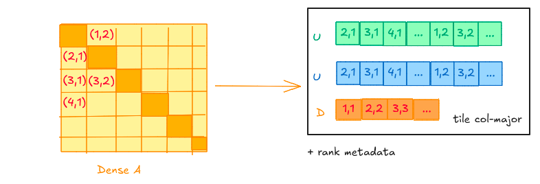
In the more general case, where we store the arrays with variable ranks, we also hold an array with the ranks \(r\) and compute its starting location in the buffer by prefix sum.
For the case the global matrix dimension \(N\) is not an exact multiple of the nominal tile size \(b\). Let
\[N = mb + b_{\mathrm{rem}},\]where \(m = \lfloor N/b \rfloor\) and \(0 \leq b_{\mathrm{rem}} < b\). If \(b_{\mathrm{rem}} = 0\), all tiles have size \(b \times b\). Otherwise, the last block row and last block column contain boundary tiles with smaller dimensions. In that case, the interior part of the matrix has dimension \(mb \times mb\), while the boundary block has size \(b_{\mathrm{rem}}\).
For this reason, it is convenient to decompose the matrix into a regular interior TLR (sub)matrix and then three boundary panels. When \(b_{\mathrm{rem}} > 0\), we write
\[A = \begin{bmatrix} A_{\mathrm{int}} & u_A \\ v_A^{T} & \gamma_A \end{bmatrix},\]where
\[A_{\mathrm{int}} \in \mathbb{R}^{mb \times mb}, \qquad u_A \in \mathbb{R}^{mb \times b_{\mathrm{rem}}}, \qquad v_A \in \mathbb{R}^{mb \times b_{\mathrm{rem}}}, \qquad \gamma_A \in \mathbb{R}^{b_{\mathrm{rem}} \times b_{\mathrm{rem}}}.\]Here, \(A_{\mathrm{int}}\) denotes the regular TLR sub-matrix formed by the full-size tiles, while \(u_A\), \(v_A^{T}\), and \(\gamma_A\) collect the boundary column, boundary row, and bottom-right corner block, respectively. So the storage becomes as in the figure below
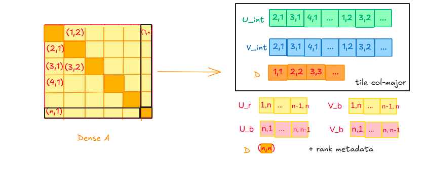
The right operand \(B\) in the TLR GEMM can have the same structure. Then the product \(C = AB\) can be written as
This decomposition separates the computation into four output regions:
\[C = \begin{bmatrix} C_{\mathrm{int}} & C_{\mathrm{right}} \\ C_{\mathrm{bottom}} & C_{\mathrm{corner}} \end{bmatrix}.\]This structure is allows to split the matrix-multiplication across terms with a regular structure, which maps well to (batched) GEMMs. The bulk of the work is the update of the interior block \(A_{\mathrm{int}} B_{\mathrm{int}}\). Moreover since, the the four ouput regions are dijsoint they can be updated concurrently on separate streams.
We explain the machinery developed to compute the interior product \(A_{\mathrm{int}} B_{\mathrm{int}}\), as this is the most computationally intensive operation and the most general. The same ideas are reused for the other products
Regular TLR GEMM
From here on we drop the \(\mathrm{int}\) subscript and work with two square interior TLR sub-matrices. The storage naturally splits each operand into its dense diagonal and its low-rank off-diagonal part, \(A = D_A + O_A\) and \(B = D_B + O_B\), so that
\[C \leftarrow \beta C + \alpha (D_A + O_A)(D_B + O_B) = \beta C + \alpha\big(D_A D_B + O_A D_B + D_A O_B + O_A O_B\big).\]The four products touch different parts of \(C_{\mathrm{int}}\):
- \(D_A D_B\) writes only the diagonal tiles of \(C\);
- \(O_A D_B\) and \(D_A O_B\) write only the off-diagonal tiles;
- \(O_A O_B\) writes both, and usually accounts for the dominant part of the work
Because the diagonal group and the off-diagonal group touch disjoint tiles, they can run concurrently on separate streams
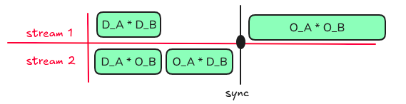
The scaling by \(\beta\) is fused into the first GEMM that writes each tile of \(C\). For a diagonal tile \(C_{ii}\), the first writer is \(D_A D_B\), so that GEMM performs
\[C_{ii} \leftarrow \beta C_{ii} + \alpha A_{ii}B_{ii}.\]For an off-diagonal tile \(C_{ij}\), the first writer is either the \(O_A D_B\) update or the \(D_A O_B\) update. That first off-diagonal GEMM uses the original \(\beta\). Every later contribution to the same tile uses accumulation mode, i.e. it is launched with \(\beta = 1\).
The easy terms
The first three products are mapped to strided batched GEMMs. The diagonal product is a batch of independent dense tile GEMMs:
\[(D_A D_B)_{ii} = A_{ii}B_{ii}, \qquad i = 1,\dots,m.\]Thus it is implemented as one strided batched GEMM with matrix size \(b \times b\) and batch size \(m\).
The product \(O_A D_B\) can be written as
\[(O_A D_B)_{ij} = U_{ij}\big(V_{ij}^{T}D_{jj}\big), \qquad i\neq j,\]and is therefore evaluated in two batched GEMM stages. Consider first the products \(V_{ij}^{T}D_{jj}\) over all off-diagonal tiles. The GEMM grouping depends on the layout of the low-rank factors. If the factors of \(A\) are stored tile-column major, then for each fixed \(j\) the matrices \(V_{ij}^{T}\), \(i\neq j\), are contiguous and can be stacked into one tall matrix. Thus the \(m-1\) products associated with column \(j\) are computed by one GEMM of size \(((m-1)r)\times b\) times \(b\times b\). Repeating this for all \(j\) gives \(m\) such GEMMs, which can be launched as one strided batched GEMM. If the factors of \(A\) are stored row-wise instead, the factors needed for a fixed \(j\) are not contiguous, so this aggregation is not available; the stage is then implemented as one small GEMM per off-diagonal tile, for a total of \(m(m-1)\) GEMMs of size \(r\times b\) times \(b\times b\).
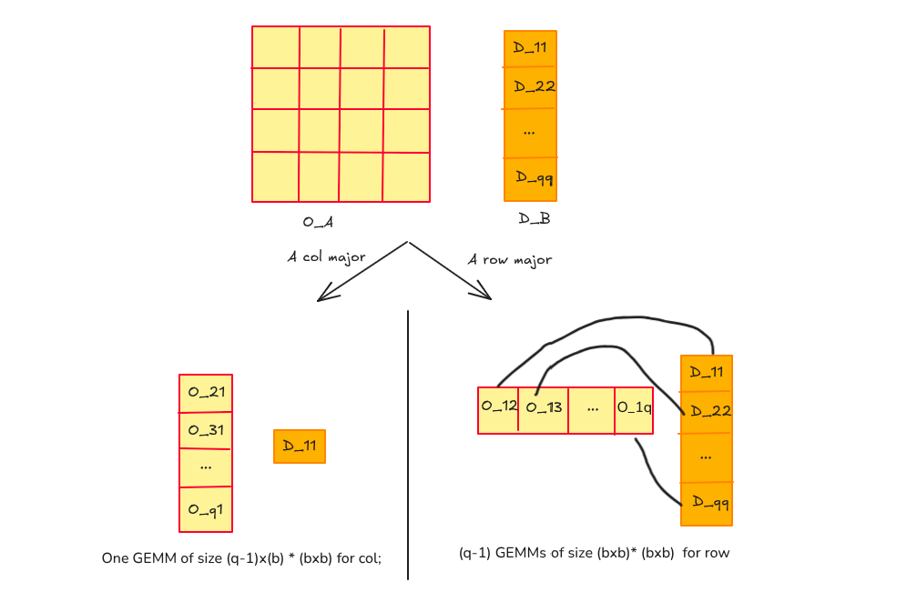
By symmetry, the opposite holds for the product \(D_A * O_B\).
The \(O_A O_B\) terms
Here both operands are low-rank. With \(\widetilde A_{ik} = U_{ik} V_{ik}^{T}\) and \(\widetilde B_{kj} = W_{kj} Z_{kj}^{T}\), the \((i,j)\) output block is
\[(O_A O_B)_{ij} = \sum_{k\neq i,j} U_{ik}\,\bigl(V_{ik}^{T}W_{kj}\bigr)\,Z_{kj}^{T}.\]We first compute the common intermediate
\[\text{Stage 1:}\qquad S_{ikj}=V_{ik}^{T}W_{kj} \in\mathbb{R}^{r_A\times r_B}.\]The remaining contractions are ordered to minimize the size of the intermediate matrix. Specifically,
- If \(r_A\le r_B\),
- If \(r_B<r_A\),
Thus, after forming \(S_{ikj}\), the multiplication order is chosen according to \(\min(r_A,r_B)\), ensuring that the intermediate matrix \(T_{ikj}\) is as small as possible.
Each stage is a collection of small GEMMs indexed by three tile indices: the output row \(i\), the output column \(j\), and the contraction tile \(k\). As in the previous section, the number and size of the GEMM depends on the layout of the factors. Every index can be handled in three cases:
- Fused into a GEMM dimension (M, N, or K): several tiles are glued into one larger matrix operand and handled by a single large GEMM. This is fastest, but requires the tiles along a given axis to be contiguous in memory
- Batched: many independent, equal-shaped GEMMs issued in one batched-GEMM call. This works for any layout, but each GEMM stays small.
- Looped serially, one GEMM per value of the index.
Fusing is best (biggest GEMMs, fewest launches), batching is the fallback for scattered data, and looping is reserved for a case we will see is unavoidable. The axes which can be fused depends on the ordering of the factors: tile column or tile major order.
The stride-1 axis
The factors are stored as \([b, r, n_{\text{off}}]\) arrays. Tiles are contiguous in memory only along the stride-1 axis, which depends on the tile layout.
| Operand | Tile-column-major | Tile-row-major |
|---|---|---|
| \(A_{ik}\) | \(i\) | \(k\) |
| \(B_{kj}\) | \(k\) | \(j\) |
This gives four possible layout combinations, which determines the optimization lever.
Lever 1: \(A\)’s layout determines how the \(k\)-sum is performed
First consider one fixed output tile \(C_{ij}\). Its low-rank update has the form
\[C_{ij} \mathrel{+}= \sum_{k\neq i,j} U_{ik}T_{ikj},\]where \(T_{ikj}\) is the intermediate produced by the previous stage. The important point is that all values of \(k\) contribute to the same output tile \(C_{ij}\). There are two ways to handle this sum:
If the factors \(U_{ik}\) are contiguous in \(k\), we can fold the \(k\)-sum into the GEMM contraction dimension. Namely, for fixed \((i,j)\) we form the block products as
\[C_{ij} \mathrel{+}= \underbrace{ \begin{bmatrix} U_{i1} & U_{i2} & \cdots \end{bmatrix} }_{b\times K_r} \underbrace{ \begin{bmatrix} T_{i1j}\\ T_{i2j}\\ \vdots \end{bmatrix} }_{K_r\times b},\]where \(K_r\) is the sum of the ranks over the contributing \(k\) indices. In this case one GEMM computes the full sum over \(k\) and writes \(C_{ij}\) once. In this case the GEMM has the schematic form. This is the write-once case for \(C_{ij}\).
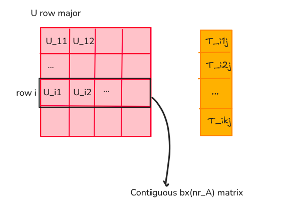
If the factors \(U_{ik}\) are not contiguous in \(k\), folding the reduction into one GEMM would require packing or copying the \(U\) panels. Without such packing, the implementation loops over \(k\):
\[\begin{cases} C_{ij} \leftarrow U_{ik}T_{ikj} + \beta C_{ij} && k=1 \\ C_{ij} += U_{ik}T_{ikj} && k=2, \dots, n-1 \end{cases}\]Now each contribution is a separate GEMM, and the same tile \(C_{ij}\) is updated repeatedly. This is the accumulate case.
Thus:
- If \(A\) is stride-1 in \(k\), then the \(U_{ik}\) panels needed for one \(C_{ij}\) are contiguous. The \(k\)-sum can be folded into the GEMM contraction dimension, and each output tile \(C_{ij}\) is written once.
- If \(A\) is stride-1 in \(i\), then the \(U_{ik}\) panels needed for one \(C_{ij}\) are scattered as \(k\) varies. The implementation loops over \(k\) and accumulates into \(C_{ij}\) multiple times.
This statement concerns one fixed output tile. Across many output tiles, we still batch or loop over the remaining free indices. For example, if the \(k\)-sum has been folded for each \((i,j)\), then different output tiles \(C_{ij}\) are independent and can be handled as a batch of write-once GEMMs. If the \(k\)-sum is not folded, then the implementation typically loops over \(k\), and for each fixed \(k\) updates a batch of output tiles \(C_{ij}\) with accumulation.
This is why the two scheduling families differ in their traffic to \(C\). In the write-once family, each \(C_{ij}\) tile is formed by a GEMM that already includes the full \(k\)-sum. In the accumulate family, each \(C_{ij}\) tile is read and written once per contributing \(k\). Since Stage 3 operates on full \(b\times b\) tiles, reducing the number of updates to \(C\) is usually the dominant consideration.
Lever 2: \(B\)’s layout determines whether Stage 1 fuses over \(j\)
Stage 1 computes \(S_{ikj}=V_{ik}^{T}W_{kj}\). For fixed \((i,k)\), the left operand \(V_{ik}^{T}\) is reused for all output columns \(j\), while the right operand \(W_{kj}\) changes with \(j\). Therefore, if the \(W_{kj}\) factors are contiguous as \(j\) varies, the products over \(j\) can be fused into the \(N\) dimension of one larger GEMM.
If \(B\) is stride-1 in \(j\), then the row-\(k\) panel
\[\begin{bmatrix} W_{k j_1} & W_{k j_2} & \cdots \end{bmatrix}\]is contiguous, and Stage 1 can compute
\[\begin{bmatrix} S_{ikj_1} & S_{ikj_2} & \cdots \end{bmatrix} = V_{ik}^{T} \begin{bmatrix} W_{k j_1} & W_{k j_2} & \cdots \end{bmatrix}.\]Thus \(j\) is fused into the GEMM \(N\) dimension. This replaces many small \(r_A\times r_B\) products by one wider GEMM.
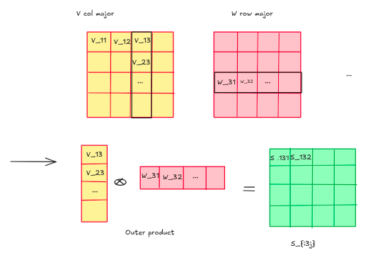
If \(B\) is stride-1 in \(k\), then the factors \(W_{kj}\) needed for fixed \(k\) and varying \(j\) are scattered. The fusion over \(j\) is not available without packing, so Stage 1 remains tilewise and is implemented as a batched GEMM.
The same idea applies to the \(i\) direction. For fixed \(k\) the factors \(V_{ik}^{T}\) are contiguous as \(i\) varies, then stage 1 can then fuse \(i\) into the GEMM \(M\) dimension.
Combining the two levers gives the four layouts:
| \(A\) stride-1 axis | \(B\) stride-1 axis | \(k\)-reduction | Stage-1 fusion | # (batched) GEMMs |
|---|---|---|---|---|
| \(k\) | \(j\) | folded into \(K\); write-once | \(j\to N\) | \(3\) |
| \(k\) | \(k\) | folded into \(K\); write-once | none; tilewise | \(3\) |
| \(i\) | \(k\) | looped over \(k\); accumulate | \(i\to M\) | \(2+n\) |
| \(i\) | \(j\) | looped over \(k\); accumulate | \(i\to M,\ j\to N\) | \(2+n\) |
Here \(n_k\) is the number of contraction tiles. The count refers to batched-GEMM launches for the \(O_AO_B\) term. In the write-once family, the computation uses three batched GEMM stages: one for Stage 1, one for Stage 2, and one for the final update to \(C\). In the accumulate family, the first two stages can still be grouped, but the final update must be performed once per contraction tile \(k\), giving \(2+n_k\) GEMM launches.
Output traversal and workspace budget
The previous discussion determines how the computation should be traversed. For each output tile \(C_{ij}\), the intermediates \(S_{ikj}\) and \(T_{ikj}\) must be stored, or at least produced in a workspace large enough to feed the next GEMM stage. With a limited workspace budget for \(S\) and \(T\), the goal is to choose the largest panel of output tiles that can be processed without spilling or excessive packing.
The best traversal depends on whether the \(k\)-reduction can be folded into the final GEMM.
In the write-once family, \(A\) is stride-1 in \(k\). For fixed output row \(i\), the factors \(U_{ik}\) are contiguous as \(k\) varies, so the whole \(k\)-sum can be folded into the GEMM contraction dimension. Thus, for a fixed row \(i\) and a block of output columns \(J\), Stage 3 has the form
\[C_{iJ} \mathrel{+}= \underbrace{ \begin{bmatrix} U_{ik_1} & U_{ik_2} & \cdots \end{bmatrix} }_{b\times K_r} \underbrace{ \begin{bmatrix} T_{ik_1J}\\ T_{ik_2J}\\ \vdots \end{bmatrix} }_{K_r\times |J|b},\]where \(K_r\) is the total rank over the contributing \(k\) indices. Increasing \(J\) increases the \(N\) dimension of this GEMM and improves throughput. Thus the natural traversal order for \(C\) is row by row. If the workspace is large enough, then several output rows \(i\in I\) can be processed at once, giving a batched GEMM over the row block \(I\).
In the accumulate family, \(A\) is stride-1 in \(i\). The axis $k$ is fused in Stage 1 and to increase the size of the GEMM we can compute \(S_{Ikj}\) for a set of rows \(I\), so the computation proceeds column-by-column. Here the key workspace decision is different. Since the final update is serial in \(k\), a deeper block of contraction indices increases the number of times the same \(C\) tile is read and written before moving on. Consequently, under a limited workspace budget, it is more effective to keep the active \(k\)-block small and allocate the remaining workspace to enlarging the free output dimension \(J\). In practice, this means fixing a single \(k\) at a time and partially updating as many \(C_{ij}\) tiles as possible, processing tile columns first
Pseudocode
The write-once (row) family, at full budget:
# A stride-1 in k  ⇒  U_ik, V_ik contiguous over k for a fixed row i
# scratch:  S[r, r, n, |J|, |I|]     T[r, n, b, |J|, |I|]

for run (block of rows I × columns J) sized to the budget:

    # Stage 1 — S_ikj = V_ik^T W_kj,  batched over (i, k, j)
    #   B stride-1 j: j fused into N   |   B stride-1 k: tilewise
    batched_gemm('T','N',  1, V[i,k], W[k,j],  0, S[i,k,j])

    # Stage 2 — T_ikj = S_ikj Z_kj^T,  batched over (i, k, j)
    batched_gemm('N','T',  1, S[i,k,j], Z[k,j],  0, T[i,k,j])

    # Stage 3 — fold k into K: one write per output row i, batched over i
    for i in I:                                 # collected into ONE batched call
        Ustack_i = [ U_i1 | U_i2 | … | U_in ]   #  b × n·r   (contiguous view)
        Tstack_i = reshape(T[i, :, :, J])       #  n·r × |J|·b
    batched_gemm('N','N',  α, Ustack, Tstack,  β=1, C[I, J])
The accumulate (column) family, at full budget:
# A stride-1 in i  ⇒  V_ik contiguous over i  (i fuses into M)
# k cannot fold into K, so it is a serial loop in Stage 3

for run (block of contraction tiles K × columns J) sized to the budget:

    # Stage 1 — batched over (k, j); i fused into M (and j into N if B stride-1 j)
    batched_gemm('T','N',  1, Vpanel[k], W[k,j],  0, S[k,j])

    # Stage 2 — batched over (k, j)
    batched_gemm('N','T',  1, S[k,j], Z[k,j],  0, T[k,j])

    # Stage 3 — the reduction: loop k, accumulate (β=1); batch the free axes (i,j)
    for k in K:
        batched_gemm('N','N',  α, U[:,k], T[k],  β=1, C[:, :])   # distinct (i,j) tiles
Benchmark
The benchmark below (not exhaustive) shows indeed that A tile-row major and B tile column major (the ij Stride-1 axis combination) results in the largest speedup
| Matrix size | Tile size \(b\) | Rank \(r\) | Dense (ms) | kj (ms) | kk (ms) | ik (ms) | ij (ms) |
|---|---|---|---|---|---|---|---|
| \(1024 \times 1024\) | 64 | 16 | 21.878 | 15.892 | 30.210 | 13.131 | 9.101 |
| \(2048 \times 2048\) | 64 | 16 | 147.426 | 119.235 | 238.657 | 96.963 | 66.572 |
| \(3072 \times 3072\) | 64 | 24 | 493.884 | 585.493 | 939.301 | 484.963 | 364.823 |
| \(2048 \times 2048\) | 128 | 32 | 148.391 | 82.159 | 100.250 | 74.737 | 64.758 |
| \(4096 \times 4096\) | 256 | 64 | 1181.113 | 488.826 | 489.062 | 479.816 | 480.066 |
| \(2048 \times 2048\) | 32 | 8 | 149.807 | 405.434 | 585.653 | 323.768 | 226.776 |