My GSoC 2025 Project with JuliaReach
21 Aug 2025Table of Contents
Outline and Motivation
In many safety-critical systems, it is often impossible to predict exactly how the system will behave due to uncertainties in initial states, inputs, or dynamics. Reachability analysis addresses this challenge by computing flowpipes that enclose all possible behaviors over time, allowing engineers to rigorously verify safety.
For example, imagine an autonomous car faced with a pedestrian suddenly stepping onto the road. Depending on its exact speed, distance to the pedestrian, and reaction delay, the car may need to brake immediately or steer around the obstacle, while also accounting for sensor errors. One could try to sample a range of initial speeds and positions and simulate the resulting trajectories to guide the decision. However, because the car’s dynamics is nonlinear even small variations in initial conditions can lead to drastically different behaviors, so simulation alone cannot provide the rigorous guarantees required for safety.
In the ReachabilityAnalysis.jl package, several algorithms are available to compute these enclosures for different types of dynamical systems with uncertain inputs and initial states, including hybrid systems.
During my project, I focused on a fundamental class of models: linear time-invariant (LTI) systems with uncertain parameters.
An LTI system describes the evolution of the state vector \(x(t)\) under a fixed matrix \(A\):
where \(x \in \mathbb{R}^n\).
Such systems are widely used because they arise naturally when linearizing nonlinear models. In practice, however, the dynamics are rarely known exactly. Parameters in \(A\) may be uncertain due to modeling errors, noisy measurements, etc.. To capture this, we consider a parametric LTI system of the form:
Here:
- \(X₀\) is the set of possible initial states, reflecting uncertainty at \(t=t_0\).
- \(\mathcal{A}\) is a set of possible system matrices, representing parameter uncertainty.
The goal is to compute a tight over-approximation of all trajectories that can arise from any choice of initial state in \(X₀\) and any admissible dynamics in \(\mathcal{A}\). This is significantly more challenging than the classical case with a fixed \(A\), since the solution space must account for both state uncertainty and dynamics uncertainty simultaneously.
Huang et al. [1] introduced a dedicated algorithm for these parametric LTI systems with uncertain dynamics, which combines two modern set representations: matrix zonotopes for modeling uncertainty in the system matrix and sparse polynomial zonotopes (SPZs) for representing the reachable states.
The motivation for this choice becomes clear when we compare possible uncertainty models for \(A\) and discuss how to best enclose the evolving states.
Why Matrix Zonotopes Instead of Interval Matrices?
A classical way to represent uncertainty in \(A\) is through an interval matrix:
\[\mathcal{A} = \{ A \mid a_{ij} \in [\underline{a}_{ij}, \overline{a}_{ij}] \}\]This representation assumes that each entry of the matrix can vary independently within its interval. While simple and well studied, this independence assumption can be overly conservative: it includes combinations of parameters that may never actually occur in practice, often resulting in loose over-approximations of the reachable set.
To address this, Althoff [2] introduced matrix zonotopes, which generalize standard zonotopes to matrices:
\[\mathcal{Z} = \{ A_0 + \sum_{i=1}^p A_i \alpha_i \;\mid\; \alpha_i \in [-1,1] \}\]Here, \(A_0\) is the center matrix, and the \(A_i\) are generator matrices. Matrix zonotopes preserve correlations between matrix entries, unlike interval matrices that treat them as independent. This leads to significantly tighter enclosures for uncertain dynamics, making them a more accurate and efficient choice in reachability analysis.
Why Sparse Polynomial Zonotopes?
Once the dynamics are modeled with matrix zonotopes, the reachable states need a representation that can handle the resulting complexity without becoming overly conservative.
Huang et al. use sparse polynomial zonotopes for this task.
SPZs extend zonotopes with polynomial terms, allowing them to capture non-convex sets while remaining closed under Minkowski sums and linear maps: two core operations in many reachability algorithms.
For a more detailed description of SPZ see [3], or for a friendly introduction, see Luca’s previous GSoC blog post
Example
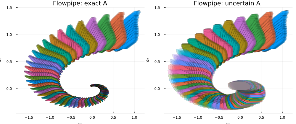
Now let’s test the algorithm with a simple 2D dynamical system:
\[x' = A x, \quad x(0) \in X_0, \quad A = \begin{bmatrix} -1 & -5 \\ -1 & -1 \end{bmatrix}.\]In this case the origin is a stable focus, since the eigenvalues are
\[\lambda = -1 \pm i\sqrt{5},\]so given an initial set \(X_0\) the trajectories should rotate and shrink towards the origin.
We then compare two cases:
- the dynamics is known exactly,
- the dynamics is uncertain.
For the uncertain case, assume that the we are unsure about one of the entries of \(A\):
\[A \in \begin{bmatrix} [-1.1, -0.9] & -5 \\ 1 & -1 \end{bmatrix}.\]This can be expressed as a matrix zonotope:
\[\mathcal{A} = \begin{bmatrix} -1 & -5 \\ -1 & -1 \end{bmatrix} + c \begin{bmatrix} 0.1 & 0 \\ 0 & 0 \end{bmatrix}, \quad c \in [-1,1].\]Now we will set up the reachability problem using LazySets and ReachabilityAnalysis:
Step 1: Import the packages
using ReachabilityAnalysis
import IntervalMatrices   # required for internal calculations
using Plots
Step 2: Define the system matrices
# Nominal matrix
A0 = [-1.0 -5.0;
       1.0 -1.0]

# Matrix zonotope with one generator
AS = MatrixZonotope(A0, [N[0.1 0.0; 0.0 0.0]])
Step 3: Define the initial set
We initialize the initial conditions as a sparse polynomial zonotope:
X0 = SparsePolynomialZonotope(
    [1.0, 1.0], # center
    0.1 * [2.0 0.0 1.0; 1.0 2.0 1.0], # independent generators
    0.1 * reshape([1.0, 0.5], 2, 1), # dependent generators
    [1 0 1; 0 1 3] # exponent
)
Step 4: Define the IVP
We can use the convenient macro @ivp to specify the initial states and uncertain dynamics:
prob1 = @ivp(x' = A * x, x(0) ∈ X0, A ∈ AS)
Step 5: Configure the reachability algorithm
We use the HLBS25 algorithm for systems with uncertain parameters:
# Time step and horizon
δ = 3 / 200
T = 3.0

# Algorithm setup
alg = HLBS25(
    δ = δ,
    approx_model = CorrectionHullMatrixZonotope(),
    max_order = 5,
    taylor_order = 5,
    reduction_method = LazySets.GIR05(),
    recursive = false,
)
Step 6: Solve and visualize
# Solve
sol1 = solve(prob1, alg; T = T)

# Plot
p = plot(X0, title="Reachable Set")
for X in sol1
  plot!(set(X), vars=(1,2))
end
This produces the flowpipe, showing how trajectories evolve while accounting for both the initial uncertainty and the uncertainty in the dynamics.
To compare with the exact case, we can repeat the experiment with a matrix zonotope that has no generators, which corresponds to a fixed matrix \(A\). The fully worked out code can be found at the end of this page in the Appendix
A not so succesful example
For small uncertainty the algorithm behaves well, but with larger uncertainty the over-approximation deteriorates. For example, if we choose a matrix zonotope with large uncertainty such as:
\[\mathcal{A} = \begin{bmatrix} -1 & -5 \\ -1 & -1 \end{bmatrix} + c \begin{bmatrix} 0.1 & 0.1 \\ 0.1 & 0.1 \end{bmatrix}, \quad c \in [-1,1].\]The results look quite bad:
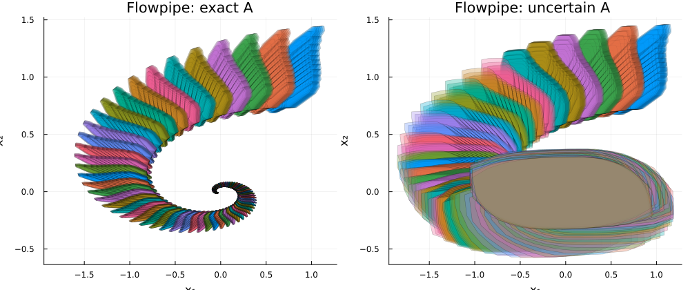
In this case we observe a very strange behaviour: the reach sets quickly bloat growing faster than they contract around the fixed poin. Interestingly, increasing the maximum order parameter seems to mitigate the bloating somewhat.
What is going wrong?
Together with my mentors, I’ve been investigating this issue for several weeks. The problem appears to stem from the repeated use of the reduce_order method. Keeping it brief, in the algorithm we compute end apply at each step the matrix zonotope exponential \(e^{\mathcal{A}}\) to propagate the state set forward in time. This increases the number of generators in the SPZ, forcing order reduction to keep the complexity manageable. However, repeated reduction seems to discard generators that capture important information, while the remaining ones grow excessively under successive exponentials.
However this is quite puzzling, since reduce_order works well in other parts of the library. At this point it is still unclear to us whether this instability reflects a deeper stability issue, perhaps some relationship between the amount of uncertainty and the step size, similar to time-stepping constraints in ODE solvers, or whether it comes from a subtle bug in the implementation of one of the many building blocks. What is certain is that the issue seems specific to this algorithm, which is still very new and, before our work, had only been implemented in the library CORA
What’s next?
After the end of the GSOC, we made a plan to further investigate the problem and finally turn the algorithm in a stable release. I have also implemented the non-homogeneous case \(x' = \mathcal{A}x + \mathcal{B}u\), however it is not ready for a release yet since there are some implementation details which require further discussion with the mentors.
Contributions Overview
In the tables below I summarize my contributions to the different packages in the JuliaReach ecosystem to implement the reachability algorithm described above.
1. LazySets.jl: Matrix Zonotopes
| PR Title | PR # | Category |
|---|---|---|
Add overapproximate for matrix zonotope exponential |
#4000 | Feature |
| Add operations on matrix zonotopes | #3999 | Feature |
Add overapproximate for matrix zonotope multiplication |
#3996 | Feature |
Preserve indexvector in linear map for MZ |
#3985 | Fix |
Extend ExponentialMap to support MatrixZonotopes |
#3970 | Feature |
Add linear_map between MatrixZonotope and SPZ |
#3969 | Feature |
Fix in-place scaling for MatrixZonotope |
#3967 | Fix |
Add methods and type for MatrixSets |
#3966 | Feature |
Add norm and overapproximate_norm for matrix zonotope |
#3941 | Feature |
Refactor and extend MatrixSets module |
#3933 | Refactor |
2. LazySets.jl: General improvements and fixes
| PR Title | PR # | Category |
|---|---|---|
Optimize remove_redundant_generators |
#3998 | Feature |
Improve remove_redundant_generators for SPZ |
#3986 | Improvement |
Add overapproximate for exponential map for SPZ and Zonotope |
#3979 | Feature |
Fix isuniversal and constructor for Polygon |
#3978 | Fix |
Preserve ID in minkowski_sum and cartesian_product between SPZ and Zonotope |
#3977 | Improvement |
Make overapproximate of ASPZ with UnionSetArray{Zonotope} more robust |
#3972 | Improvement |
Add overapproximation of the l1 norm of a Zonotope |
#3925 | Feature |
Faster l1 norm for AbstractZonotope |
#3924 | Improvement |
Add scale for SPZ |
#3908 | Feature |
Add merge_id and generalize exact_sum for SPZ |
#3905 | Feature |
| Add sampler for sparse polynomial zonotopes | #3847 | Feature |
3. MathematicalSystems.jl and ReachabilityAnalysis.jl
| PR Title | PR # | Notes |
|---|---|---|
Add parametric systems |
#332 | Feature |
| Add HLBS25 algorithm for linear parametric systems | #931 | Feature |
References
[1] Yushen Huang, Ertai Luo, Stanley Bak, Yifan Sun, Reachability analysis for linear systems with uncertain parameters using polynomial zonotopes, Nonlinear Analysis: Hybrid Systems, Volume 56, 2025, 101571, ISSN 1751-570X. DOI
[2] Matthias Althoff, Reachability Analysis and its Application to the Safety Assessment of Autonomous Cars, PhD thesis, Technische Universität München, July 2010.
[3] Niklas Kochdumper, Matthias Althoff, Sparse Polynomial Zonotopes: A Novel Set Representation for Reachability Analysis, IEEE Transactions on Automatic Control, Vol. 66, No. 9, Sept. 2021, pp. 4043–4058. DOI
Appendix
using ReachabilityAnalysis
import IntervalMatrices
using Plots
N = Float64

A0 = N[-1 -5;
        1 -1]
AS = MatrixZonotope(A0, [zeros(2,2)])

# Initial set
X0 = SparsePolynomialZonotope(
    N[1.0, 1.0],
    N(0.1) * N[2.0 0.0 1.0; 1.0 2.0 1.0],
    N(0.1) * reshape(N[1.0, 0.5], 2, 1),
    [1 0 1; 0 1 3]
)

# Two problems: no variation vs. small generator variation
prob1 = @ivp(x' = A * x, x(0) ∈ X0, A ∈ AS)

AS = MatrixZonotope(A0, [N[0.1 0.1; 0.1 0.1]])
prob2 = @ivp(x' = A * x, x(0) ∈ X0, A ∈ AS)

δ = N(3) / 200
T = 3.0

alg = HLBS25(
    δ = δ,
    approx_model = CorrectionHullMatrixZonotope(),
    max_order = 5,
    taylor_order = 5,
    reduction_method = LazySets.GIR05(),
    recursive = false,
)

sol1 = solve(prob1, alg; T = T)
sol2 = solve(prob2, alg; T = T)

# plotting function
function plot_flowpipe(sets, X0; kwargs...)
    p = plot(; kwargs...)
    for (i,s) in enumerate(sets)
        if i%3 ==0
            plot!(p, set(s); vars=(1,2), alpha=0.3, lw=0.5)
        end
    end
    return p
end

p1 = plot_flowpipe(sol1, X0,
    title = "Flowpipe: exact A",
    xlabel = "x₁", ylabel = "x₂",
    legend = true)

p2 = plot_flowpipe(sol2, X0,
    title = "Flowpipe: uncertain A ",
    xlabel = "x₁", ylabel = "x₂",
    legend = true)

# common limits for better comparison
xlims_common = (min(xlims(p1)..., xlims(p2)...), max(xlims(p1)..., xlims(p2)...))
ylims_common = (min(ylims(p1)..., ylims(p2)...), max(ylims(p1)..., ylims(p2)...))
plot!(p1; xlims=xlims_common, ylims=ylims_common)
plot!(p2; xlims=xlims_common, ylims=ylims_common)

plot(p1, p2, layout=(1, 2), size=(1000, 420))
savefig("reach_comp.png")